Digital illustration of a bar chart displayed on a whiteboard. The graph features alternating blue and orange bars representing data points in a professional, educational context.

Digital illustration of a box plot diagram on a white background. The chart displays statistical data quartiles labeled Q1, Q2 (median), and Q3 along a horizontal scale.

Why we study this

Data Handling

Types of statistical charts, Histograms, Mean Mode and Median, Standard Deviation and Interquartile Range, Sampling Methods

Digital illustration of a colorful pie chart used to visualize data categories like Maths, Science, English, and Other. The layout is clean and minimalist with a clear legend alongside the segmented chart.

'Lies, damned lies and statistics!' is a well-known quote often attributed to the English Prime Minister Benjaming Disraeli. Statistics can't lie, but their interpretation can be distorted, as pointed out in Darrell Huff’s 'How to Lie with Statistics' , a humorous guide to spotting how misleading samples, averages, graphs, and percentages can distort the truth. The book encourages readers to question how statistics were collected and presented before accepting them.

How do we make truthful sense of data? By selecting a graph, chart or diagram which suits the nature of the data, and draws out the salient features. The art of choosing the right graph, chart or diagram is often called Exploratory Data Analysis (EDA). This developed as statisticians began looking beyond formal tests to understand data through careful observation and visualisation. John Tukey played a leading role in establishing EDA as a distinct approach, especially through his 1977 book Exploratory Data Analysis, which promoted plots, summaries, and flexible questioning to reveal patterns, unusual values, and relationships before drawing conclusions.

History of Data Handling

William Playfair introduced early bar, line, and pie charts in the late 1700s.
J. F. W. Herschel and Francis Galton helped develop scatter diagrams in the 1800s.
Florence Nightingale (1820–1910) used her coxcomb chart to show that preventable disease killed more soldiers than battle wounds, helping persuade leaders to improve hospital sanitation.
Marie Neurath (1898–1986) helped turn statistics into clear pictorial charts and infographics.
Karl Pearson introduced the term histogram in 1891.
John Tukey — popularised box plots, stem-and-leaf plots, and Exploratory Data Analysis in the 1970s. He also helped to coin the words 'software' and 'bit'.

A famous example of the wisdom of crowds comes from Francis Galton. At a 1906 livestock fair, about 800 people guessed the weight of an ox. Many guesses were far off, but the average was remarkably close to the true weight. The story shows how a large group can sometimes produce a surprisingly accurate estimate, even when individual guesses vary widely.

1786

Playfair’s early charts made data visual.

1833–1880s

Scatter diagrams revealed relationships.

1891

Pearson introduced the term histogram.

Galton’s ox story showed the wisdom of crowds.

1906

Tukey formalised Exploratory Data Analysis.

1977

Florence Nightingale

(1915–2000)

John Tukey (1915–2000)

Data Handling Exam Tips

Studio photography of a young man at a desk, focused on writing in a notebook. He has a calm, studious demeanor in a bright and tidy home office setting.

Different types of data require different handling. Category data does not need to be numerical. Numerical data divides into discrete or continuous. Data one counts is discrete; data one measures is continuous. But discrete doesn't mean 'integral': if you record the proportion in a finite sample, this is discrete as well.

Techincally this has to do with being countable. Real numbers are uncountable: try to put them into an ordered list and you will never exhaust them. Fractions are actually countable: you can devise a way of counting them which captures them all.

Two types of infinity: countable and uncountable!

Types of statistical charts

Bar Chart

Best for: Comparing discrete categories (e.g., sales per month, population by country).

Structure: Rectangles with lengths proportional to the values they represent, with spaces between bars.

Line Graph:

Best for: Tracking changes, trends, or continuous developments over time (time series data, such as monthly revenue or daily temperature

Structure: Data points plotted on a coordinate plane and connected by straight line segments.

temperature).

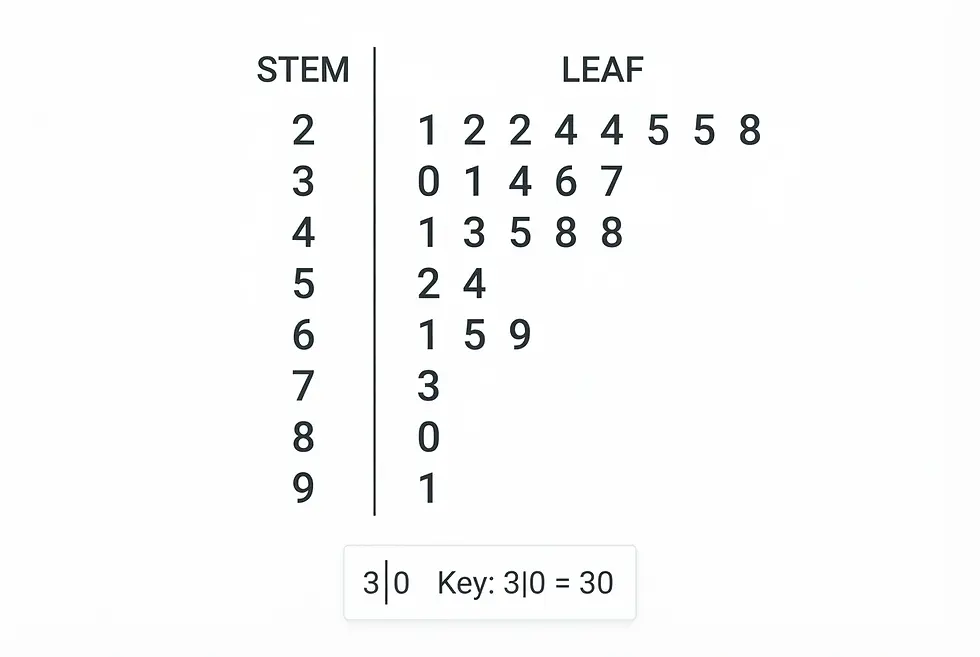
Digital diagram showing a stem-and-leaf plot with grouped numerical data. The chart is clean, minimalist, and educational in style.

Stem-and-leaf diagram

Best for: Discrete data sets. The leaves indicate the shape of the distribution. Remember to add a key - the data in the above could be 2.1, 2.2, ... or 0.21, 0,22, ... The key gives the order of magnitude. The raw data is preserved in the diagram

Box-and-whisker diagram

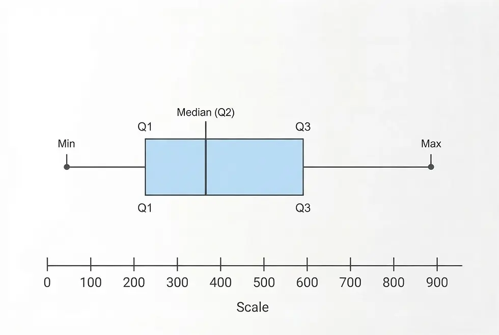
Best for: Displaying the summary statistics of a dataset—minimum, lower quartile, median, upper quartile and maximum

Structure: A box representing the middle 50% of the data (Interquartile Range) with lines ("whiskers") extending to the extremes.

Histogram:

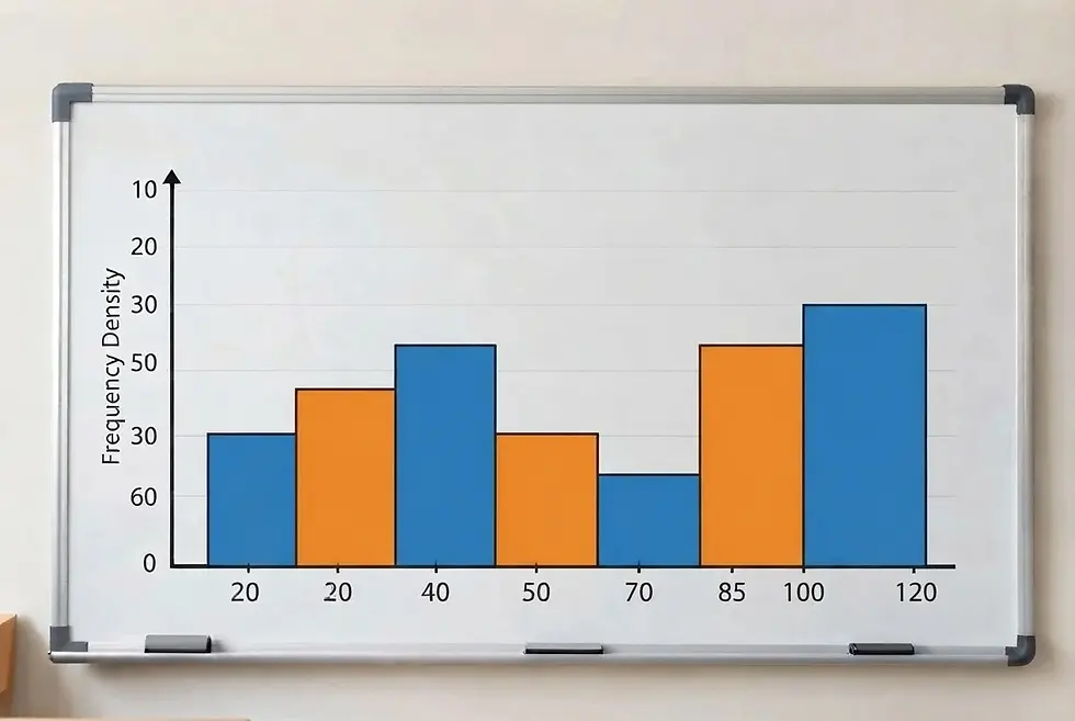
Best for: Showing the frequency distribution of continuous numerical data grouped into range intervals (bins), such as exam scores or ages. Linear scale on horizontal axis, frequency density on vertical axis. Area of bars represents frequency

Structure: Similar to a bar chart, but the bars touch each other to represent continuous data.

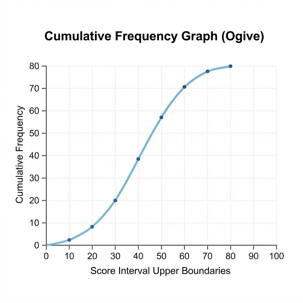
Digital chart showing a cumulative frequency ogive graph. The S-shaped curve illustrates frequency accumulation against score intervals.

Cumulative frequency curve

Best for: Showing the cumulative frequency of a grouped frequency distribution. The median and quartiles, and amount of data above or below given values, can be estimated.

Structure: Plot the cumulative frequencies against the endpoints of the intervals.

Pie chart

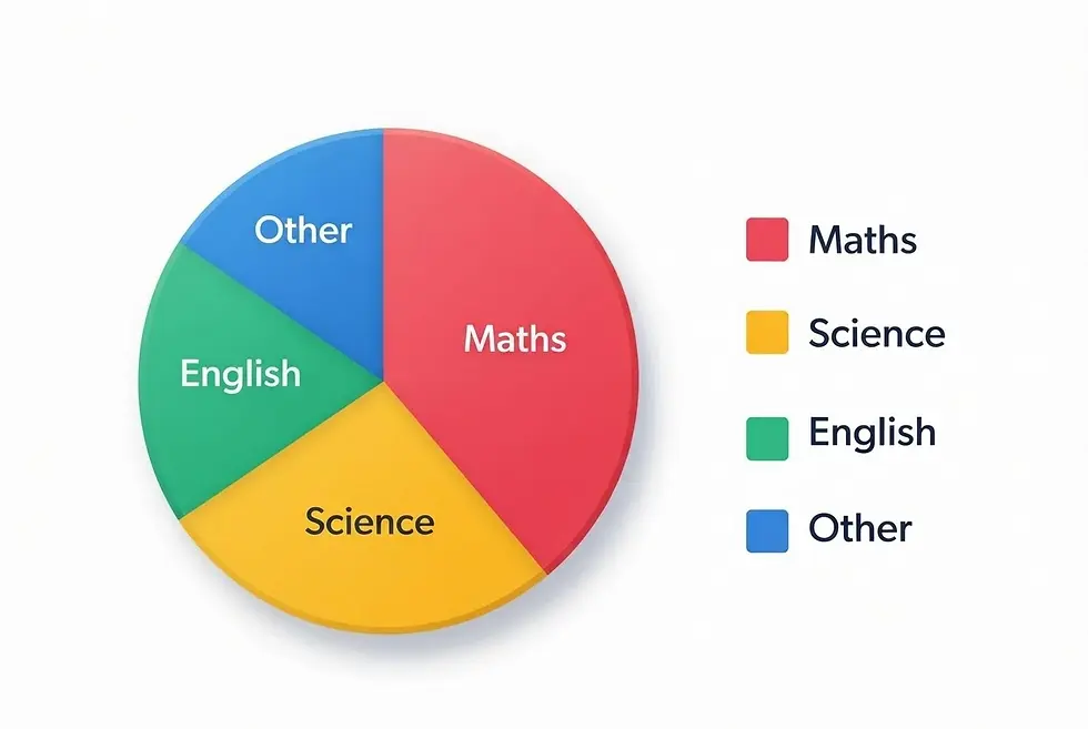
Best for: Showing parts of a whole (percentages) when you have 3 to 6 categories

Structure: A circle divided into slices proportional to each category's share of 100%.

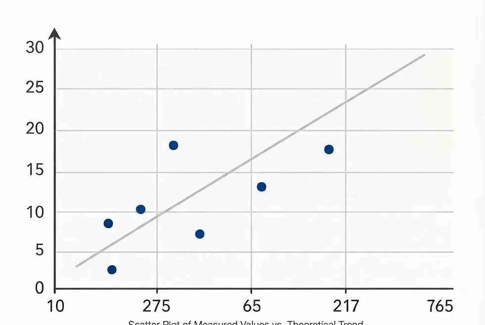
Scatter Plot:

Best for: Showing the relationship or correlation between two numerical variables (e.g., height vs. weight).

Structure: Individual points mapped along two axes without connecting lines.

Histograms

Histograms look like bar charts but are fundamentally different. The vertical axis contains frequency density, which is frequency divided by class width. This means the frequency is represented by the area if the bars. The horizontal axis should be a scale, and as this is for continuous data there shold be no gaps between the bars.

A histogram allows for different sizes of 'bin'. The mean value will divide the histogram into equal areas.

Be careful with class widths! If data is rounded to the nearest unit then a 10 to 19 bin has effective limits of 9.5 to 10.5, so the class width is 10, not 9. Similarly, ages 10 to 19 have limits of 10 and 20, as ages are rounded down, and the class width is 10.

Question: draw a histogram for the following data:

Class

Frequency

0 < x ≤ 10

10 < x ≤ 20

20 < x ≤ 40

40 < x ≤ 50

Outliers

There are two definitions of outliers. In terms of quartiles and Interquartile range (IQR), anything above the upper quartile plus 1.5 x the IQR or below the lower quartile minus 1.5 x the IQR is regarded as an outlier.

In terms of mean and standard deviation (SD), the boundaries are above mean + 2x SD and below mean - 2 x SD.

Mean, mode, median

Suppose a small company has 4 employees earning £25,000 and the managing director on £100,000, which is an outlier. The median salary is £25,000, whereas the mean is (4x25000+100000)/5 = £40,000. So the median is less affected by outliers. The mode is also £25,000, but is not really relevant for a small set of data. For a grouped fequency distribution, the midpoints of the classes are used, so the mean is an estimate only.

Interquartile range and standard deviation

The interquartile range is not affected by the top quarter of bottom quarter of the data, so again is less affected by outliers than the standard deviation, which is calculated using all the values. For a grouped frequency distribution, the midpoints are used to calculate the standard deviation, so this is again only an estimate.

Mean and standard deviation formulae

For data without frequencies:

Mean: x̄ = (Σx) / n

Variance = Σ(x − x̄)² / n = Σx²/n - x̄²

Population standard deviation: σ = √[Σ(x − x̄)² / n]

For a frequency distribution:

Mean: x̄ = (Σfx) / (Σf)

Variance = Σf(x − x̄)² / n = Σfx²/n - x̄²

Population standard deviation: σ = √[Σf(x − x̄)² / (Σf)]

Here, f is the frequency, x is each value or class midpoint, x̄ is the mean, n is the number of values, and Σf is the total frequency.

Standard deviation with divisor n - 1

When sample data is used to estimate the standard deviation of a population, we use a divisor of n - 1 instead of n in the formulae when calculating an estimate of the population standard deviation. This is because this is an unbiased estimator: using a divisor of n under-estimates the population standard deviation because it measures deviations from the sample mean x̄ rather than the population mean μ, and x̄ is itself based on the sample values.

Most calculators give two possible values for σ; the larger one is calculated with a divisor of n - 1.

Calculating Medians and quartiles

For small data sets: Order the data, then if there are n of them calculate m = (n + 1)/2, rounding down if needed. If n is odd then the median is the mth item. If n is even then take the average of the mth and (m+1)th.

For the lower quartile and upper quartile repeat the same procedure for m = (n + 1)/4 and m = 3(n + 1)/4.

For frequency distributions: Plot a cumulative frequency curve, using the endpoints of each 'bin'. Then split the total frquency into quarters and read off the corresponding values.

Types of sample

It is important to select samples which are free from bias, both in the way the sample is selected and the way questions in questionnaires are framed. The sample must be representative of the population. In politics, pre-election polls usually use samples of about 1500 voters, a very small fraction of the voting population. A margin of error can be calculated when the sample is randomly selected. The larger the sample, the smaller the theoretical error. But things can go wrong...

Example: the 2015 UK general election

Most opinion polls predicted a close contest or a hung Parliament, but the Conservatives won a majority. An official inquiry found that the samples did not represent some groups of Conservative voters well enough. This shows how an unrepresentative sample can produce misleading results.

Sampling method

Simple random

Stratified

Quota

Systematic

Cluster

Opportunity

How it works

Every member has an equal chance of selection (technically every sample of size n is equally likely, but this boils down to the same thing).

Divide the population into groups, then sample proportionally from each group. This ensures that every group is represented.

Select a set number from each group, without necessarily using random selection.

Choose every nth member after a random starting point.

Divide the population into groups and randomly choose whole groups.

Sample from data which is to hand or convenient.

Return to Advanced maths topics